Generation of high-frequency topographic Rossby waves in the Gulf of Mexico

1 Introduction

A number of societal factors motivate the need for improved forecasting and a better understanding of Gulf of Mexico Loop Current (LC) system dynamics: extensive energy sector operations in the Gulf, rapidly intensifying tropical storms in response to warming Gulf waters, sea level rise along the densely-populated Florida coast and downstream impacts on the Gulf Stream (Hirschi et al., 2019). The LC dominates upper-layer circulation in the Gulf. It enters through the Yucatan Channel and exits through the Florida Straits, evolving from a port-to-port mode to an extended mode, penetrating up over the Mississippi Fan. Occasionally, the LC pinches off and sheds a large 200 – 400 km Loop Current Eddy (LCE) which can detach and reattach multiple times before a final separation and subsequent westward translation across the Gulf. The deep layers of the eastern Gulf (>1000 m) have been characterized as relatively quiescent during the port-to-port mode. In contrast, when the LC advances, the deep circulation is energized through topographic interactions and LC instabilities (Donohue et al., 2016).

In the early 1990s, oil and gas operators recognized that bursts of strong deep currents arrive along the deep continental slope without warning. Prompted by this risk to operations, a series of observational studies were funded by Minerals Management Service, now Bureau of Ocean and Energy Management (BOEM) to directly measure and diagnose these deep currents. Hamilton (1990) attributes these strong bottom-intensified fluctuations with frequencies between 1/40 – 1/20 days^–1 to topographic Rossby waves (TRWs). Coherence between sites suggests a westward propagation with group velocity of about 9 km day^–1 hypothesized to originate under LC meanders over the Mississippi Fan. Hamilton and Lugo-Fernandez (2001) builds upon this work using observations from Sigsbee Escarpment where lower-layer variability is found to be higher frequency (1/20 – 1/10 days^–1) and exceptionally more energetic than in other regions of the deep Gulf.

Oey and Lee (2002) establishes a direct link between the LCE separation process and TRWs by using a numerical simulation of the Gulf of Mexico. Deep variability is consistent with observations with spectral peaks in the 1/100 – 1/20 day^–1 frequency band. This work identifies regions where a sufficient topographic slope to support the propagation of TRWs coincides with both bottom intensification and significant eddy kinetic energy in the equivalent periodicity band. Energy paths produced by a TRW ray-tracing model align with these TRW active regions along the northern slope of the Gulf and, when traced backward, are found to originate under the LC and LCEs. This work establishes the LC as an energy source for TRWs propagating along the northern slope of the Gulf of Mexico.

A major finding from numerical results is the funneling of ray paths towards the Sigsbee Escarpment (Oey and Lee, 2002), resulting from the presence of deep currents and wave refractions over steep topography. This region therefore plays an important role in determining downstream propagation as refraction will alter wave characteristics and can locally intensify the currents. Observations of lower-layer currents at the escarpment are made by Hamilton (2007) using an array of five moorings deployed along and just straddling the slope. High energy fluctuations typical of TRWs with dominant frequencies of 1/14 – 1/8 days^–1 and maximum speeds nearing 100 cm s^–1 are measured with high coherence along and at the base of the escarpment. Only very high energy events are able to penetrate inshore of the escarpment, confirming that steep topography acts as a barrier by refracting and possibly reflecting high-frequency energy back into the deep Gulf. Another significant result from Hamilton’s work is a relatively persistent, yet distinct series of wave trains traveling through the escarpment, all with unique frequencies occurring during different stages of the LC shedding process. This provides evidence that energy transfer can occur under a number of dynamic conditions and originate from many locations across the eastern Gulf.

While ray tracing evinces a link between the LC and TRWs (Oey and Lee, 2002; Hamilton, 2007), the dynamics by which that energy transfers to lower layers remains an outstanding question. A complicating factor is that deep energy likely originates from many different locations around the eastern Gulf. A relatively well documented process is the generation of deep energy through baroclinic instabilities in growing upper layer Loop Current meanders during LCE separation. Below the main thermocline, this eddy kinetic energy (EKE) manifests as anticyclones and cyclones with frequencies in the 1/100 – 1/40 day^–1 band (Donohue et al., 2016). A number of studies attribute the radiation of energy away from the baroclinic instability regions to westward propagating TRWs. Oey (2008) uses a high resolution numerical model to study the generation of deep eddies by baroclinic instabilities, concluding that TRWs are excited by a simple linear eddy-wave coupling mechanism over shoaling topography. Hamilton (2009) argues that observed coherence between upper and lower layer relative vorticity fluctuations in the 1/35 – 1/20 day^–1 frequency band, where the lower layer leads upper meanders by a 90° phase offset, is characteristic of a baroclinic instability mechanism. Further evidence is provided by Hamilton et al. (2019) who use an aggregate of floats in the Gulf to observe a significant increase in deep EKE generated intermittently by meanders of the LC and LCE detachments, similar to what is observed by Donohue et al. (2016). They argue that radiation of this energy through TRWs is supported by observations of large amplitude, rectilinear oscillations just west of a retracting LC or departing LCE.

A hypothesis of TRW generation suggests that LC interactions with topography triggers a transfer of energy to the lower layer, generating perturbations through potential vorticity adjustments over a sloping bottom depth (Malanotte-Rizzoli et al., 1987; Hamilton, 1990). Viable topographic features in the Gulf of Mexico include the Mississippi Fan and the continental slope surrounding West Florida Shelf and Campeche Bank. This mechanism is thought to generate energy across a broad range in frequencies and is frequently proposed as a TRW forcing mechanism in the Gulf owing to observations of characteristic motion with frequencies spanning 1/100 – 1/10 days^–1 Hamilton, 1990; Hamilton and Lugo-Fernandez, 2001; Hamilton, 2007). A similar mechanism that likely works in concert with LC pulsations over topography is a potential vorticity adjustment in response to a squashing of the lower layer by an advancing LC front. Hamilton et al. (2019) observes a number of anticyclones north of the Campeche Bank that intensify under the northward extension of the LC and dissipate once the LC becomes stationary or retreats. They hypothesize that deep anticyclones are dispersed into radiating TRWs once the lower layer compression stops but are unable to detect the radiation from observations.

Another deep energy generation mechanism that has been proposed to radiate TRWs in the Gulf is an upper-lower layer resonant coupling first described by Malanotte-Rizzoli et al. (1995). This theory suggests that deep energy will be generated by an upper layer meander that has a frequency and wavenumber that projects onto the TRW dispersion relation local to the bottom slope and stratification. Resulting lower layer flows will couple to the upper, generating TRWs of equivalent frequency and wavelength that are free to propagate away from the coupling region. Pickart (1995) shows this is a viable generation mechanism for TRWs observed by a mooring array off Cape Hatteras. Offshore of this region, Gulf Stream meanders are predominantly eastward, so in order for coupling to occur, strongly sloped bathymetry must be oriented in a northerly (meridional) direction to generate an eastward component of phase speed at depth. Observed 1/40-day^–1 TRWs are traced backward to a region of the Gulf Streamwhere the most commonly occurring meanders have a matching frequency and fit one component of the dispersion relation. In the Gulf of Mexico, meanders in the LC are analogous to the Gulf Stream and while many studies have proposed this theory as a TRW generation mechanism, none have been able to identify the coupling and subsequent propagation.

While observations of the deep circulation in Gulf of Mexico have increased substantially, a number of questions related to TRW pathways and generation mechanisms remain unanswered. An array of 24 bottom mounted current and pressure recording inverted echo sounders (CPIES) located across the eastern Gulf of Mexico is ideally positioned to address a number of these unknowns. This array, funded by the National Academies of Science, Engineering and Medicine under the Understanding Gulf Ocean Systems initiative (UGOS), was deployed from June 2019 to May 2021 and expanded to the north, west, and south beyond the BOEM funded Observations and Dynamics of the Loop Current (DynLoop) PIES array recovered in 2011. This work will focus on propagation and generation mechanisms of the high-frequency (1/20 – 1/10 day^–1) energy observed by the array.

2 Data and methods

The array consists of 24 CPIES mounted on the seafloor in the central Gulf of Mexico (Figure 1) for nearly two years, June 2019 - May 2021. Extending from 25°N to 27.5°N, 86°W to 89°W, instruments are spaced approximately 60 km apart, a distance chosen based on known correlation length scales from previous Gulf experiments. The array allows for mapping of the circulation at mesoscale resolution and its size is designed to cover the entire LCE detachment area while expanding upon the DynLoop PIES array recovered in 2011 (Hamilton et al., 2015).

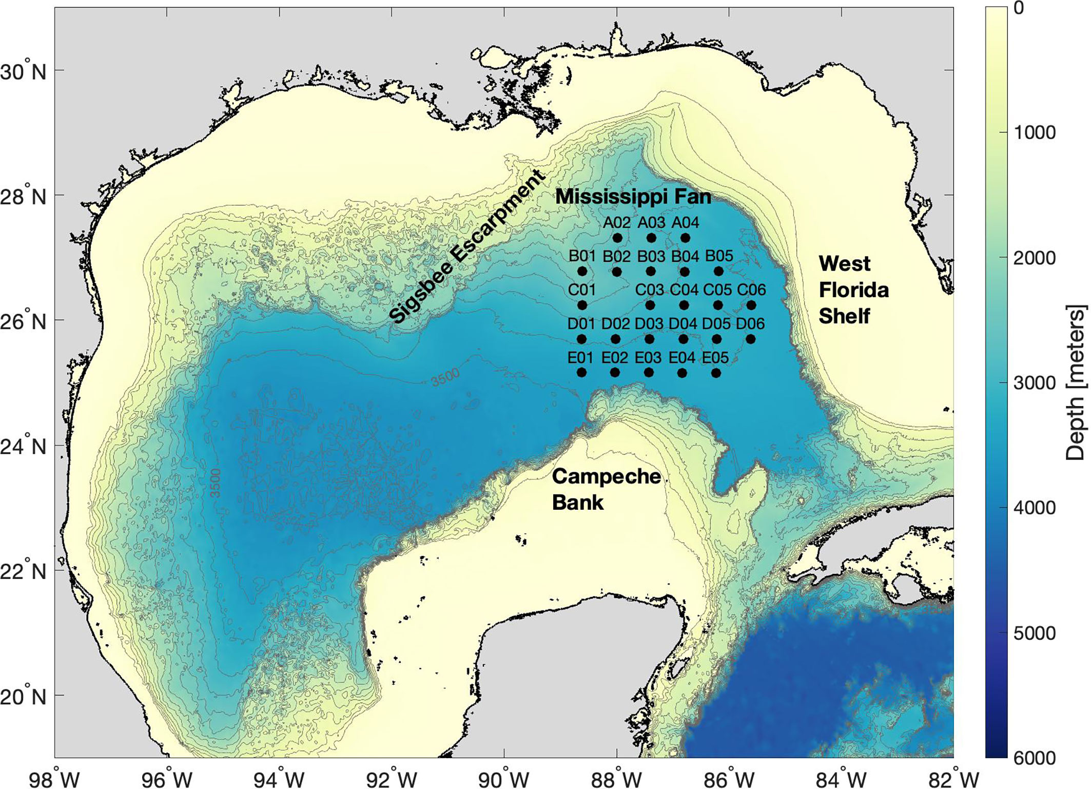
Figure 1 The Understanding Gulf Ocean Systems array comprised of 24 CPIES deployed June 2019 and recovered May 2021 in the eastern Gulf of Mexico. Locations of the CPIES are denoted by black circles and labeled. Bathymetry is contoured every 250 meters.

The inverted echo sounder emits a sound pulse at 12 kHz and measures the acoustic round trip travel time from the sea floor to the surface and back, τ (Watts and Rossby, 1977). Using empirical relationships developed with historical hydrography, tau provides an estimate of the vertical temperature, salinity and density structure. The IES was configured for four pulses every 10 minutes and data are processed through a two step windowing and median filtering process to get hourly measurements (Kennelly et al., 2022). Housed within the instrument, a pressure gauge measures bottom pressure every 30 minutes. Tidal signals are removed following Munk and Cartwright (1966) and pressures are dedrifted and leveled to the same geopotential surface as in Donohue et al. (2010). As in Donohue et al. (2010) a basin wide signal, termed common mode, is removed. Both τ and pressure are 72-hour low pass filtered and subsampled at 12-hour increments.

Current magnitude and direction are measured outside the bottom boundary layer at 50 m from the seafloor. Samples are taken every 30 minutes. The record is corrected for the local magnetic declination and the sound speed applicable to each instrument depth. Corrected zonal and meridional velocities are subsequently 72-hour low pass filtered and subsampled at 12-hour increments. A thorough description of CPIES instrumentation, data processing, τ -derived fields and mapping techniques may be found in Donohue et al. (2010) and, for PIES in the Gulf, Hamilton et al. (2015)

To convert τ measurements to profiles of temperature, salinity and specific volume anomaly, we utilize the Gravest Empirical Mode (GEM) representation (Meinen and Watts, 2000). The GEM exploits the relationship between the integrated speed of sound to known profiles of temperature and salinity from historical hydrography to create a look up table for measured τ values. Detailed treatment of the Gulf of Mexico GEM can be found in Hamilton et al. (2015) and Donohue et al. (2016). The Gulf of Mexico GEM was originally established for the Exploratory Study of Deepwater Currents in the Gulf of Mexico (Donohue et al., 2006) expanded upon for the DynLoop study (Hamilton et al., 2015) and now expanded upon further for the UGOS Initiative. Previously, the hydrographic data set accumulated for the Gulf of Mexico GEM consisted of 1136 casts, extending to at least 1000 dbar and representing about 30 years of sampling (Hamilton et al., 2015). The most recent update includes 98 CTD casts taken during deployment, telemetry and recovery and an additional 9984 Argo profiles spanning 2003 to 2021. The GEM is now based upon 11218 hydrocasts, of which more than 4400 extend to 2000 dbar.

Absolute sea surface height is calculated by summing a reference level sea surface height, SSH_ref, with a baroclinic sea surface height, SSH_bcb. Reference level sea surface height is bottom pressure divided by gravity and bottom density: SSH_ref = P_ref/ρ_bg. Baroclinic sea surface height is geopotential height referenced to zero at the bottom divided by gravity, where geopotential is estimated from measured τ and the empirical lookup table for specific volume anomoly: SSH_bcb = ϕ_bcb/g. Together we obtain the absolute sea surface height as

This calculation of sea surface height from CPIES has been shown to compare well to a long track altimetric SSH anomaly data in the Gulf of Mexico (Hamilton et al., 2015; Donohue et al., 2016). SSH_ref and SSH_bcb are mapped at 12-hour intervals using objective analysis techniques (Bretherton et al., 1976). For this application, bottom pressure maps are created using inputs from both pressure and near-bottom velocities (Watts et al., 2001). This multivariate optimal interpolation approach constrains pressure and velocity to be geostrophic and the addition of the velocity sharpens gradients. As described in Hamilton et al. (2015), two-stage mapping is applied to both SSH_ref and SSH_bcb. For SSH_ref , first a 20-day low-passed field is mapped with correlation length scale of 70 km. Then an anomaly field is mapped with a correlation scale of 65 km. For SSH_bcb, the data are first 40-day low passed and mapped with a 170 km correlation length scale and the anomaly is mapped with a 60 km correlation length scale.

Near real time sea surface height data from Copernicus Marine Service provide a wider regional context of the upper-ocean circulation during the study period. The gridded altimeter product is estimated by optimal interpolation, merging data from all altimeter missions: Jason-3, Sentinel-3A, HY-2A, Saral/AltiKa, Cryosat-2, Jason-2, Jason-1, T/P, ENVISAT, GFO, and ERS1/2. This global mapped daily product has 25 km horizontal resolution. In this product, the position of the LC is indicated by a single 0.65 cm contour, a SSH value closely aligned with the edge of the LC. This contour is used to calculate Loop Current area, a metric used to quantify the extension of the LC into the Gulf. Detachment of LCEs is identified as a breaking of the 0.65 cm SSH contour and an abrupt decline in LC area.

3 Regional circulation June 2019 – May 2021

Three LCEs, Sverdrup Thor and Ursa, separate from the core of the LC during the CPIES deployment. The final detachment of Eddy Sverdrup occurs just days into the deployment and thus only a small portion of the LCE separation process is observed. We therefore mainly focus on the subsequent two LCE separations, Eddy Thor and Eddy Ursa. While both LCEs eventually separate and propagate off to the west, the events are notably distinct in a number of ways. This includes the number of preliminary detachments, pinch off locations, position of large meanders in both the LC and on the periphery of detached eddies and the generation and propagation of deep energy across the array. To illustrate these differences during the LC separation events and highlight the relationship between upper layer fluctuations and deep energy, maps of SSH_ref (deep pressure scaled as sea surface height) and LC position are plotted at five to eight day intervals spanning the time of LC advancement to final separation (Figures 2, 3).

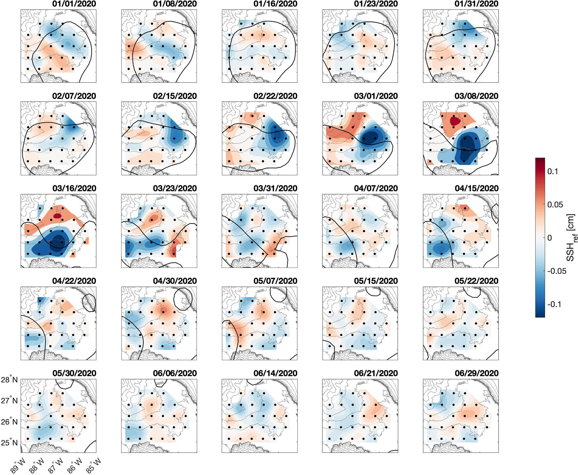
Figure 2 Mapped deep pressure fields, SSH_ref, at seven to eight-day intervals during LCE Thor shedding event, January-June 2020. The bold SSH contour represents the location of the LC. CPIES locations are marked by black circles and bathymetry is contoured in light gray every 250 meters.

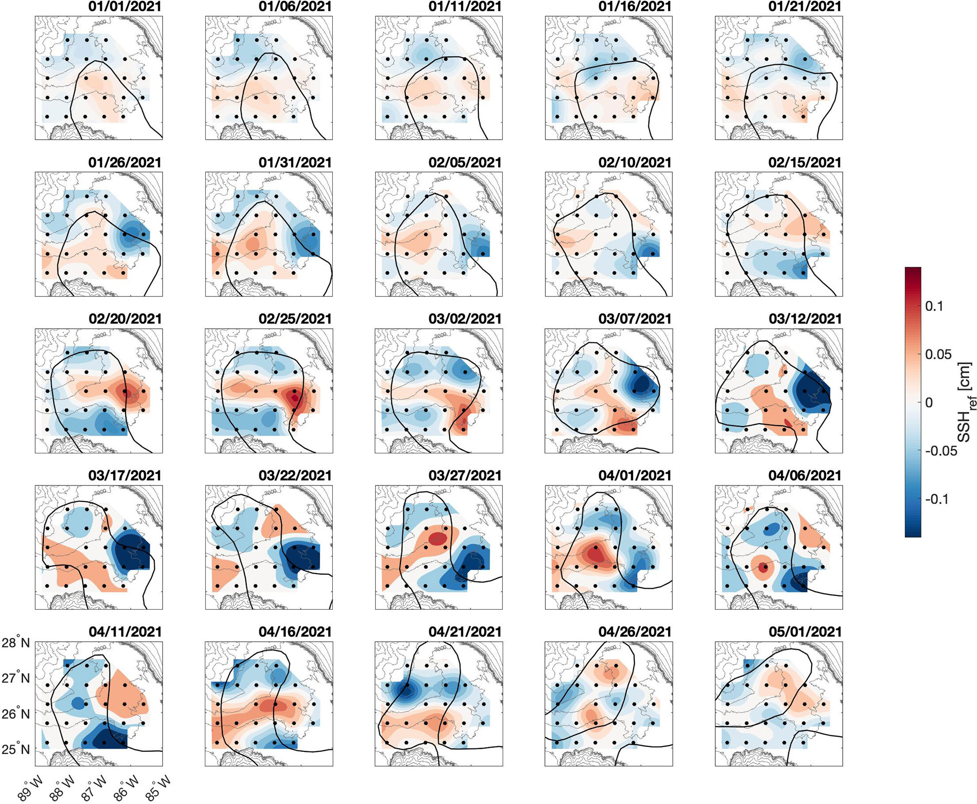
Figure 3 Mapped deep pressure fields SSH_ref at five-day intervals during LCE Ursa shedding event, January-May 2021. The bold SSH contour represents the location of the LC at each time step. CPIES locations are marked by black circles and bathymetry is contoured in light gray every 250 meters.

3.1 Eddy Thor: January to July 2020

The LC extends into the central Gulf and over the Mississippi Fan until the first detachment of LCE Thor in mid-to-late January, 2020 (Figure 2). During this period, a few small amplitude perturbations are observed in the deep fields with some indication of topographically controlled propagation; note the progression of a low pressure band from northeast corner of the array from January 1st - January 8th. Nevertheless, deep energy remains weak during the first detachment and reattachment. Perturbations intensify after the first detachment of Thor which occurs to the south of the array in early February. During this time, a sizable meander appears along the northern edge of the LCE which continues to grow even after the LCE reattaches in mid-March. Beneath the meander trough, a deep cyclone intensifies and is accompanied by a strengthening anticyclone, indicating deep energy generation presumably through baroclinic instability. These deep perturbations begin to dissipate in late March followed by the final separation of LCE Thor, which pinches off in the southeast corner of the array and quickly propagates off to the west and outside the array. A small surface anticyclone is shed from the LC in mid-April once the LCE has fully separated. It propagates along the West Florida Shelf, just outside the periphery of the array and does not appear to generate any notable perturbations in the deep. By mid-June, Thor has propagated away, the LC has retracted and the deep returns to a nearly quiescent state.

3.2 Eddy Ursa: January to May 2021

The LC propagates onto the Mississippi Fan in January, 2021 and remains in the extended state until it begins to pinch in on itself in early February (Figure 3). During this time, deep fields are fairly quiescent with a small amplitude cyclone intensifying under the meander trough associated with the necking down phase of the separation. This deep low travels southward under the meander until it propagates outside the array. In late February, an anticyclone appears under this eastward arm of the LC just downstream of the meander crest, a possible indication of a brief baroclinic instability setup before the LC pinches in on itself in early March. The LCE briefly detaches, during which a larger amplitude cyclone begins to form under the eastern side of the eddy. The amplitude of this perturbation continues to grow while it remains relatively in place and the LCE reattaches. For the remainder of the study period, the LC is characterized by large fluctuating meanders. In the deep, the large amplitude cyclone propagates southward beneath the meander trough and is eventually accompanied by a strong anticyclone in late March. This setup precedes the development of a steep meander in the LC which initiates a pinching off phase until the end of our study period when the array is recovered in early May. During this time, amplitudes of the deep perturbations are decreasing as these layers of the eastern Gulf return to their relatively quiescent state.

4 Deep energy distribution

In the eastern Gulf the LC and the detachment of LCEs are the main suppliers of energy to the deep, generating deep EKE through baroclinic instabilities and forcing TRWs along the continental slope. The CPIES array captures the generation of deep EKE, calculated as $\frac{1}{2}(u{\text{'}}^2+v{\text{'}}^2)$ where primes denote deviation from the time mean, under the mean position of the eastward arm of the LC (Figure 4A). Time-averaged EKE peaks between approximately 25°– 27°N, 86°– 87°W, similar but slightly west of what was observed by Donohue et al. (2016). A band of slightly intensified EKE extends out along 26°N suggesting a pathway of deep energy propagation. The time-averaged velocity field also identifies similar features to Donohue et al. (2016), including a deep cyclone centered near 26.8°N, 86°W, slightly north of previous observations, and a broad anticyclonic circulation around 26°N, 87.6°W. Another cyclone is centered near 26.9°N, 88°W, a region outside the bounds of the previous array. The influence of LCE separation events on deep energy is evident from the array-averaged deep EKE, peaking during each detachment (Figures 4B, C). During the first few days of deployment, Eddy Sverdrup separates from the LC corresponding to a sharp decline in energy, followed by a slower decline over the subsequent months. The formation of Thor is unique as the deep EKE fields remain weak as the LC advances and Thor detaches for the first time. It seems likely that the deep EKE generated during the first detachment isn’t captured within the array as the detachment point is south of the array. Deep EKE does peak just prior to reattachment and declines again after the final separation. During LCE Ursa formation, deep energy increases during the first necking-down phase of separation and remains high throughout the remainder of the study period.

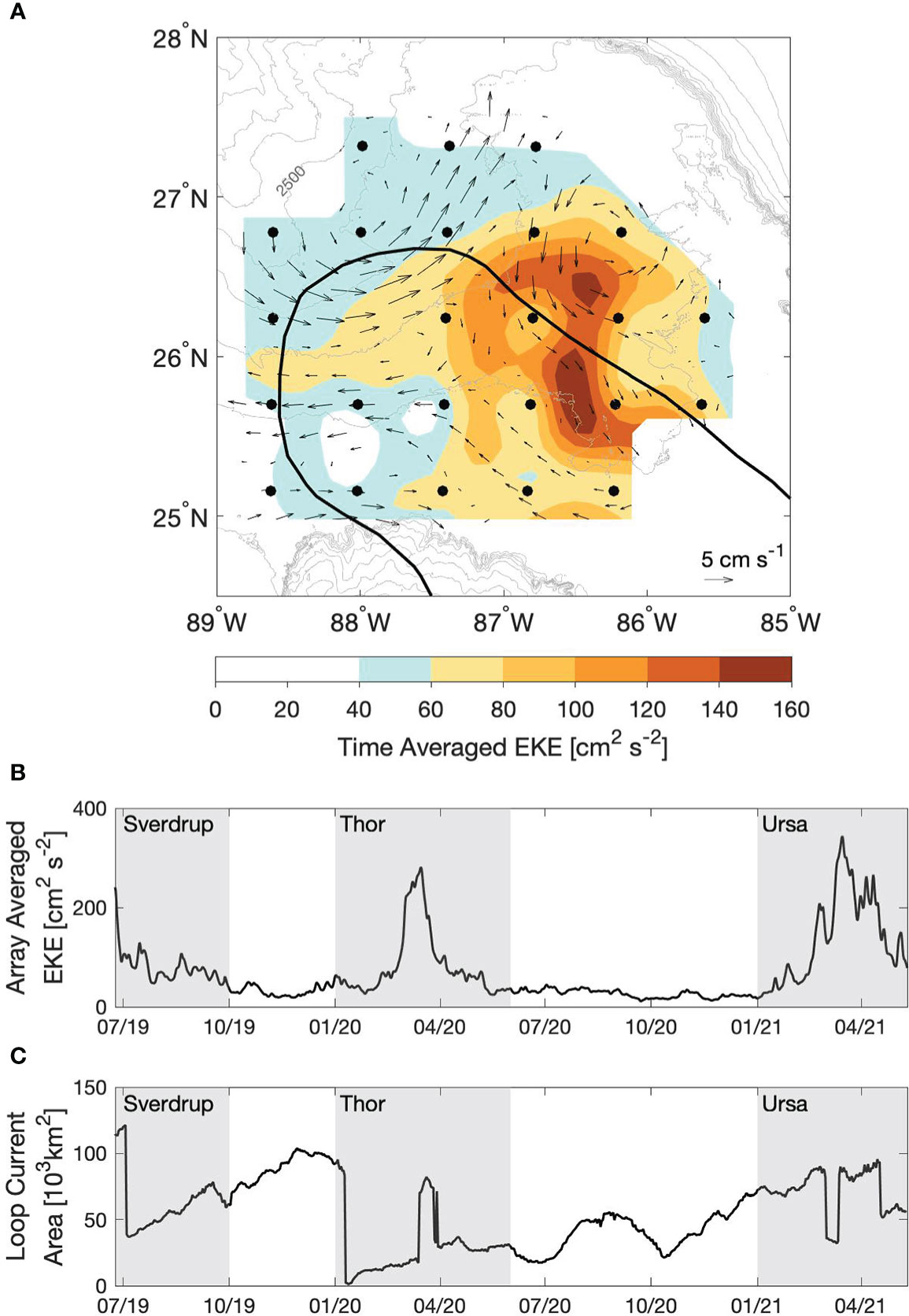
Figure 4 Deep eddy kinetic energy and current vectors (A), time averaged over the study period. The bold SSH contour represents the mean position of the LC. CPIES are denoted by black circles and bathymetry is contoured in gray every 250 meters. The array-averaged eddy kinetic energy (B) is compared against the LC Area (C), derived from satellite SSH. Formation time-frames for LC Eddies Sverdrup, Thor and Ursa are highlighted by gray boxes.

The spectral content of energy generated in the deep layers of the Gulf is found to vary across the array, organized into two distinct frequency bands (Figure 5). The southeastern region of the array is dominated by low frequency fluctuations within the 1/100 – 1/20 day^–1 band and devoid of energy at higher frequencies. Much less low frequency energy is found in the northwestern portion of the array which is instead characterized by a distinct peak between 1/20 – 1/10 days^–1. Motivated by these discrete spectral bands of SSH_ref, the distribution of variance is mapped as a function of frequency (Figure 6). While nearly an order of magnitude smaller, spatial variance in the 1/100 – 1/20 day^–1 band reflects that of the total distribution. Variance peaks near 26°N, 86°W, centered slightly east of the region of maximum EKE and north of the mean position of the LC. Another region of enhanced low frequency variance is also found along the southeast edge of the array. This overall pattern is similar to what was identified by Donohue et al. (2016) and attributed to deep eddies generated by instabilities under meanders of the LC. In contrast, a band of high-frequency (1/20 – 1/10 day^–1) variance is found along the base of the Mississippi Fan while almost no variance is found in the southeast corner of the array where the low frequencies had maxima. Maximum variance in the 1/20 – 1/10 day^–1 band is about an order of magnitude smaller than that of the low frequency, with maximum values near 26.2°N, 88.4°W.

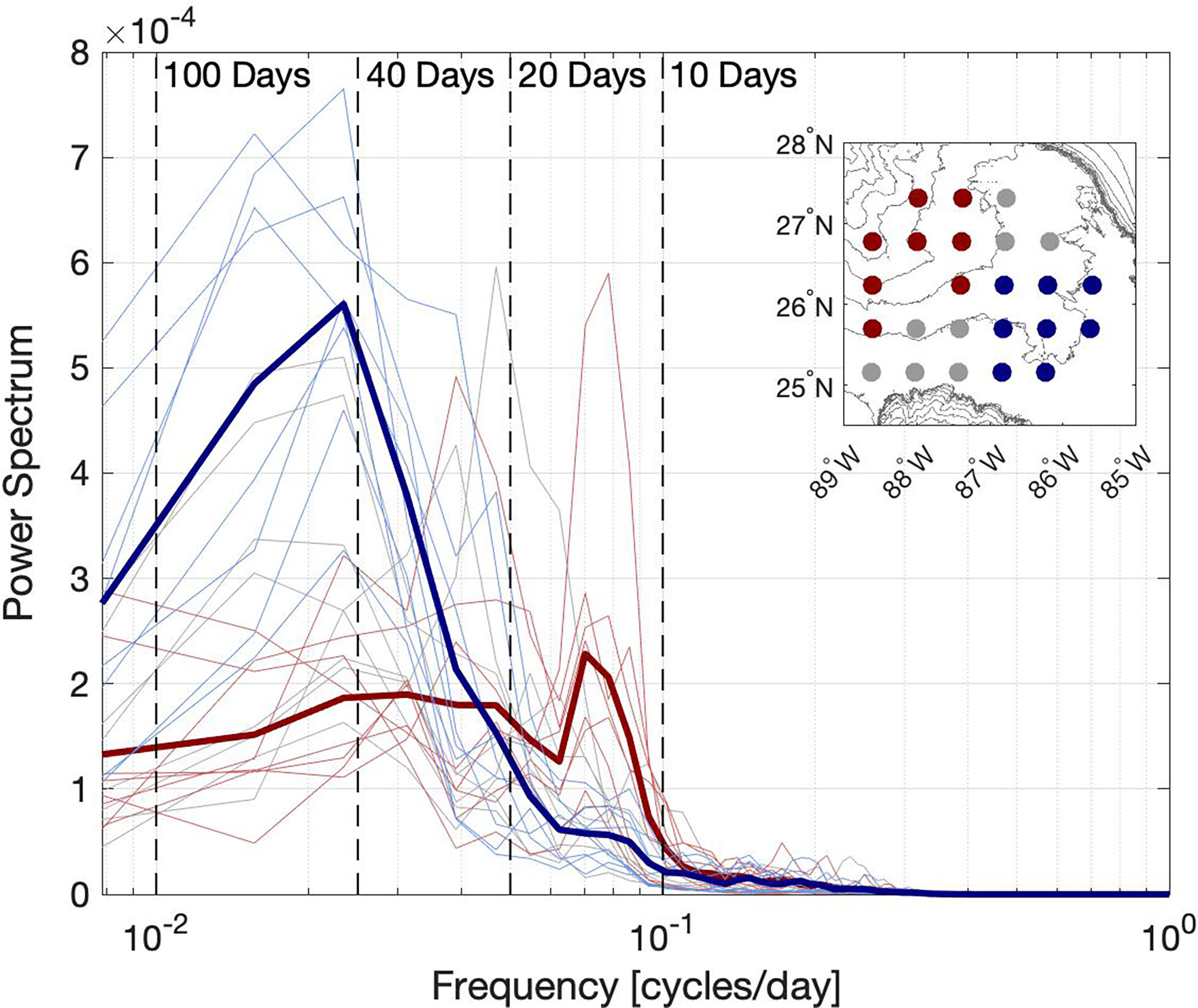
Figure 5 Variance-preserving spectra for CPIES bottom pressures, SSH_ref in the southeastern (blue) and northwestern corner of the array (red). Remaining instruments are in gray. Individual instruments are in light shades and area averages are in dark bold colors. Frequency limits, labeled by their corresponding period, are denoted by dashed vertical lines. Inset identifies sites in the southeastern (blue), northwestern (red) and remaining groups.

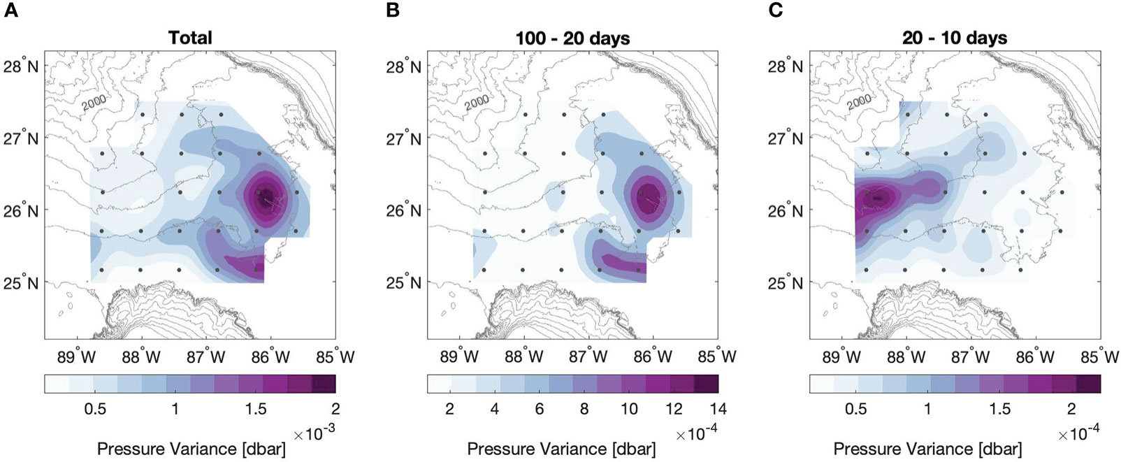
Figure 6 Deep pressure variance across all frequency bands (A), in the 1/100 – 1/20 day^–1 frequency band (B) and in the 1/20 – 1/10 day^–1 frequency band (C). Variance range is unique to each panel, decreasing from left to right. CPIES locations are marked by black circles and bathymetry is contoured in light gray every 250 meters.

We focus here on the deep high-frequency energy which did not receive attention in previous DynLoop studies. We hypothesize that the band of SSH_ref variability along the base of the Mississippi Fan is representative of propagating TRWs. Energetic TRWs within this frequency band have been shown to dominate deep current variability at the Sigsbee Escarpment and, when traced backward are found to radiate from this region of high variability (Hamilton, 2007). These new UGOS observations progress further and indicate, as shown next, that TRWs can originate within the LCE formation region and propagate towards the escarpment.

5 Deep energy radiation

To diagnose the origin of observed high-frequency spatial variability propagating along the base of the Mississippi Fan, we consider characteristics of TRWs derived from the dispersion relation and linear wave equations. TRWs are bottom trapped, meaning the amplitude of fluctuations increases with depth and is strongest just outside the bottom boundary layer. The degree of bottom trapping is inversely proportional to the wavelength, stratification and bottom slope (e.g. Pickart, 1995). Phase and group velocity in the northern hemisphere are to the right of increasing water depth, with phase velocity mainly along the direction of increasing water depth. Group velocity is roughly perpendicular to phase velocity, generally oriented along bathymetric contours. TRWs are refracted by a change in the magnitude of bottom slope such that group velocity trends slightly upslope in regions of weak bottom slope, and alternatively is more nearly along the bathymetry in regions of steeper slope.

While the instruments do not provide any vertical information to identify evidence of bottom trapping, the horizontal resolution of the CPIES array allows us to explore phase and group characteristics in relation to bathymetry. A complex EOF analysis (CEOF) is used to diagnose dominant spatial and temporal patterns of the high-frequency propagation across the array. The CEOF is applied to the full two-year record of 1/20 – 1/10 day^–1 band-passed SSH_ref to produce a normalized spatial amplitude, phase propagation and temporal amplitude coefficients (Figure 7). Propagation is in the direction of increasing phase and is only plotted in regions where the normalized spatial amplitude is greater than 0.3. A similar use of a Hilbert transform to compute CEOFs from a scalar field can be found in Trenberth and Shin (1984). We focus exclusively on the first mode, accounting for 51% of the variance.

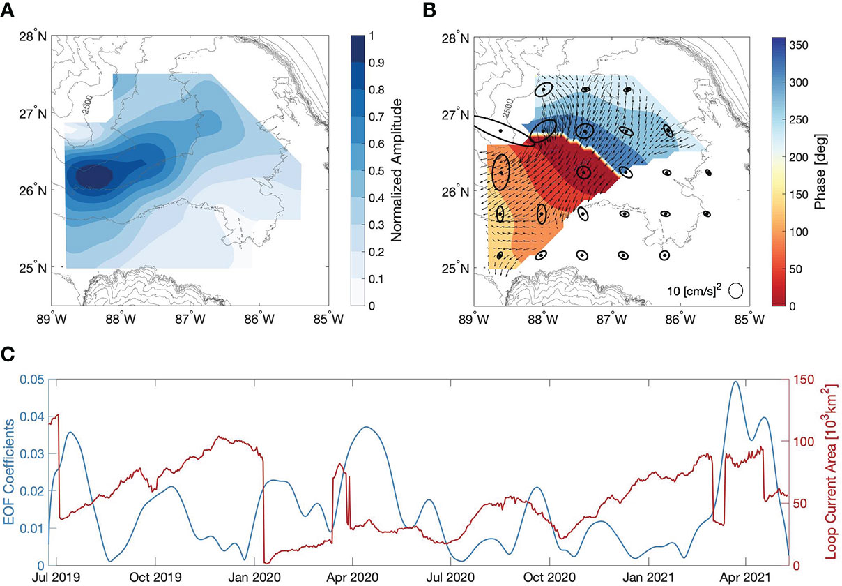
Figure 7 Normalized spatial amplitude (A) and phase in degrees (B) derived from CEOF of 1/20 – 1/10 day^–1 band-passed reference sea surface height, SSH_ref, during the full two year deployment. Phase is plotted for regions where the spatial amplitude is greater than 0.3. Propagation direction indicated by the phase gradient (arrows). CPIES locations are marked by closed black circles surrounded by 1/20 - 1/10 day^-1 band-passed variance ellipses. Bathymetry is contoured every 250 meters. CEOF amplitude time series (C; blue) and LC Area (C; red) derived from satellite altimetry.

The normalized spatial amplitude (Figure 7A) identifies a propagation pathway similar to what is observed by the high-frequency variance distribution (Figure 6C). Propagation is from the northeast corner of the array to the southwest, bending around the topography of the Mississippi Fan. Amplitude is the highest along the western side of the array, near 26.2°N, 88.4°W. The phase gradient illustrates the magnitude and direction of phase propagation across the array. The largest phase speeds are found along the northern side of the array where the bathymetric slope begins to steepen along the Mississippi Fan. In a narrow region near 88.0°W (sites A02 and B02) propagation is to the south-southeast, turning westward along the band of highest amplitude and slowing as it approaches 88.7°W along the western side of the array. Variance ellipses of the 1/20 - 1/10 day^-1 band-passed near bottom velocities at each CPIES site again illustrate how little high-frequency energy is found in the southeast corner of the array. In contrast, in the northwest corner, ellipses are rectilinear with the principal axis generally oriented along the bathymetry.

We identify a number of characteristics from the high-frequency CEOF that agree with TRW linear ray theory. The phase propagation around the Mississippi Fan in the region of significant spatial amplitude is clearly oriented with shallow water to the right. Within this region, over the steepening bathymetric slope of the Mississippi Fan, the maximum TRW frequency, ω ≥ (N│Δh│)/tanh(Nhk/f), is 1/10 days^–1 and therefore able to support these high frequency observations. In contrast, maximum frequencies in the southeast corner of the array, where observed 1/20 – 1/10 day^–1 variance is weak, range from 1/30 – 1/40 days^–1 owing to the more gradual bathymetric slope. Within the high amplitude region, we also identify a number of CPIES sites where the direction of phase propagation is oriented perpendicular to the principal axis of the independently measured variance ellipses, confirming a plane-wave like propagation. Additionally, the steepest bathymetric slope coincides with the largest phase speeds in the northern portion of the array around 27°N, 88°W. Here, we find phase direction oriented more offshore and variance ellipses roughly aligned with bathymetry. Approximate wavelengths of 150 – 300 km with phase speeds of 10 – 12 km d^–1 are estimated from the phase gradient, values consistent with both linear wave theory and observations of TRWs with frequencies in the 1/100 – 1/10 day^–1 range in the Gulf of Mexico.

The time series of EOF coefficients (Figure 7C) illustrates peaks in high-frequency energy are closely associated with the LC cycle, where an abrupt decline in LC area indicates a shedding event. We find three major peaks in 1/20 – 1/10 day^–1 energy, each following a LCE formation event, in July 2019, April 2020 and March – May 2021. This suggests the LCE shedding process is responsible for generating high-frequency TRWs. We also find a peak in high-frequency energy near Jan-Feb 2020, after the first separation of LCE Thor. The area-averaged EKE, dominated by low frequencies, did not have a peak at this time (Figure 4). Additional smaller peaks are found throughout the study period, such as Oct 2019 and Oct 2020, appearing to be dissociated with the LCE separation process and sometimes occurring when the LC is in a retracted state. These remotely-generated TRW wave trains could arise from LC interaction with topography or baroclinic instabilities that occur outside the array.

6 Deep energy generation

It is well understood that energy injected into the deep Gulf by the LC propagates along the northern continental slope as TRWs (Oey and Lee, 2002; Hamilton, 2007; Hamilton, 2009). The dynamics by which energy is transferred to the deep remains difficult to observe, a consequence of numerous generation mechanisms that can act in different locations across the eastern Gulf. Baroclinic instabilities under the eastward meandering arm of the LC has been shown to generate significant eddy kinetic energy in the deep (Donohue et al., 2016), produced by a forced upper/deep coupling. The process by which this energy reorganizes and radiates into freely propagating TRWs remains to be understood. It has been proposed that these deep eddies organize into TRWs through linear eddy-wave coupling (Oey, 2008), and while observations have not confirmed this process, Hamilton et al. (2019) uses characteristic Lagrangian float behavior to argue that energy is radiated away from the baroclinic instability regions as TRWs. Deep eddy generation through potential vorticity adjustments in response to LC advancement over the Mississippi Fan or compression of the lower layer by the LC front has been shown to produce deep energy in numerical models (Le Hénaff et al., 2012) and in float observations (Hamilton et al., 2019). Energy radiation by TRWs is hypothesized but not confirmed by observations. Finally, an upper-lower layer resonant coupling has been shown to generate TRWs originating from eastward meanders in the Gulf Stream (Pickart, 1995). Numerous studies have speculated that meanders of the LC, analogous to the Gulf Stream, should generate TRWs, however observations have not yet confirmed this coupling.

Unlike observations of TRWs, which have been confirmed across the Gulf, observations of their generation mechanisms are much more difficult. Few studies have conclusively linked generation to propagation, a consequence of the difficulty in observing these episodic and non-stationary processes by moorings and Lagrangian floats. Our array, ideally situated across the eastern Gulf of Mexico, is at an advantage to capture the transfer of energy and subsequent propagation of these bottom trapped waves.

We focus here on deep energy generation during the period of LCE Ursa formation and detachment. We focus only on a single time period for a few reasons: 1) the Ursa detachment produces the highest amount of energy in the 1/20 – 1/10 day^–1 frequency band, 2) generation and propagation appears local to the array during this time period, 3) previous detachments generate deep energy across and outside the array with high variability in both time and space and 4) by focusing on a single time period we aim to isolate a single generation mechanism.

During LCE Ursa formation, the first advancement of the LC onto the Mississippi Fan does not generate strong fluctuations in the 1/20 – 1/10 day^–1 frequency band (Figure 8). It is not until the first necking-down phase of separation, sometime around February 20th, that small amplitude perturbations are observed around the western perimeter of the LC. These perturbations increase in magnitude over the next few days corresponding to the initial detachment of LCE Ursa. Following reattachment on March 12th, deep, high-frequency fluctuations intensify under a strong meander of the LC in the northeast corner of the array and propagate as wave-like (alternating high-low SSH_ref) perturbations to the west-southwest around the Mississippi Fan. This pattern continues through the second necking down phase, until around April 21st when the eastern arm pinches in on itself over the southern portion of the array. The pattern of propagation from the northeast corner of the array resembles that of Figure 7, suggesting this high-frequency energy can be attributed to TRWs.

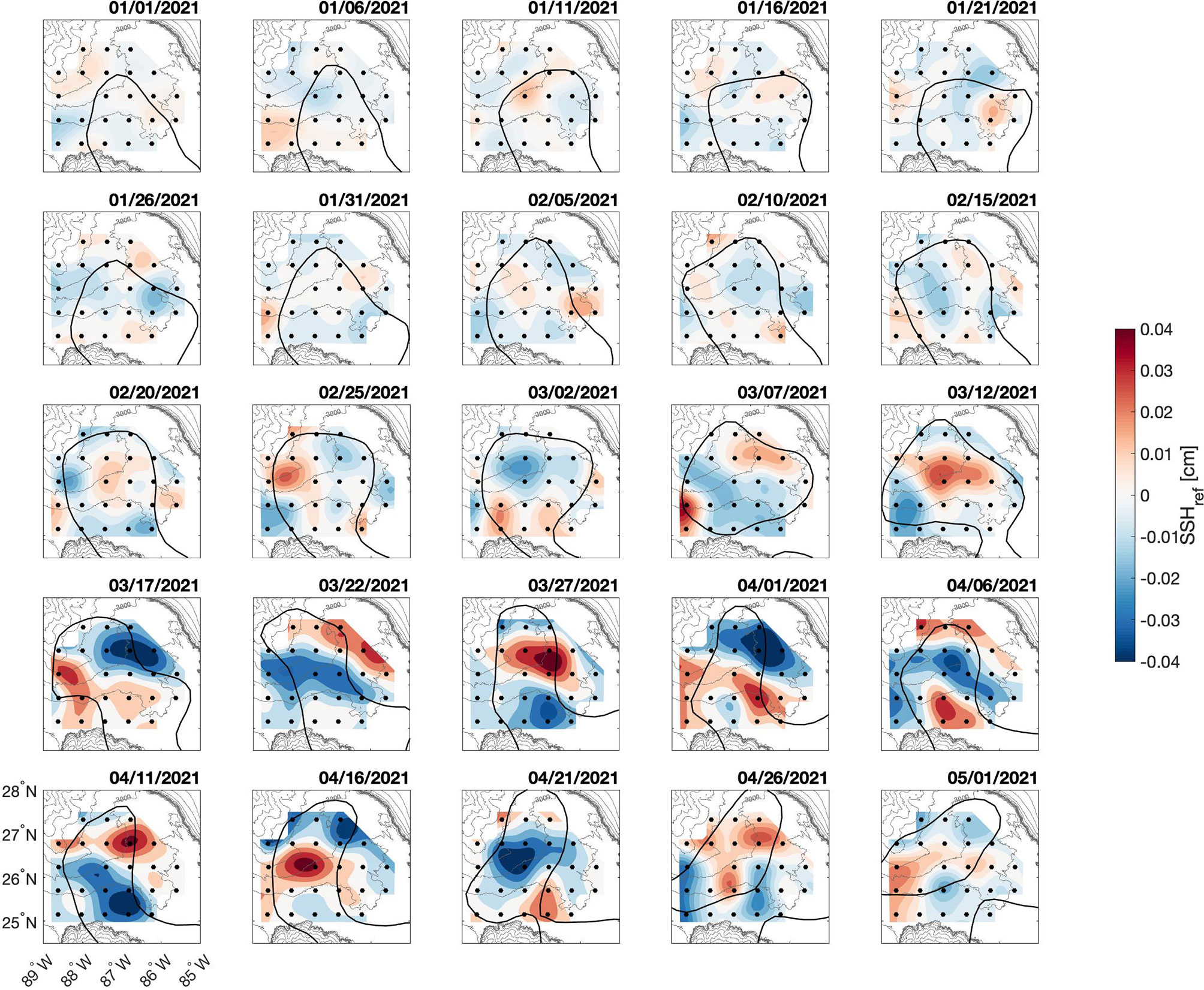
Figure 8 Mapped SSH_ref at five-day intervals during LCE Ursa shedding event, January-May 2021. SSH_ref is band-passed with a 1/20 – 1/10 day^–1 filter. The bold SSH contour represents the location of the LC at each time step. CPIES locations are marked by black circles and bathymetry is contoured in light gray every 250 meters.

A coupled upper and lower layer CEOF calculated during the time period of LCE Ursa formation and separation (January – May 2021) is used to illustrate cohesive fluctuations and phase propagation jointly in upper ocean meanders and deep perturbations. The upper field is represented as SSH_bcb and the lower as SSH_ref. Both full time series are band-passed filtered in the 1/20 – 1/10 day^–1 frequency band, scaled by their respective variance and concatenated into a single input for the CEOF. The output is remapped into the four panels shown in Figure 9. In the upper layer, we find highest spatial amplitudes (Figure 9A: dark gray) around the perimeter of the LC and the briefly detached LCE Ursa (LC position plotted in purple in the upper panels). The phase (Figure 9B) follows the same pattern, propagating anticyclonically around the LC. In the lower layer (Figure 9C), a clear propagation path is observed from the northeast corner of the array, bending around the Mississippi Fan and exiting the array around 26.5°N. A peak in deep spatial amplitude is also found to the south near 25.4°N, 86.8°W. Phase propagation (Figure 9C) is generally southwest in the high amplitude region around the Mississippi Fan. The blue highlighting in Figures 9A, B identifies areas where fluctuations in both the upper and the lower layers have coincident heightened amplitude. The observations demonstrate coherent motion in both layers. The coherence in this region is also confirmed by direct squared coherence and wavelet cross spectra, all showing the same phase offsets (not shown).

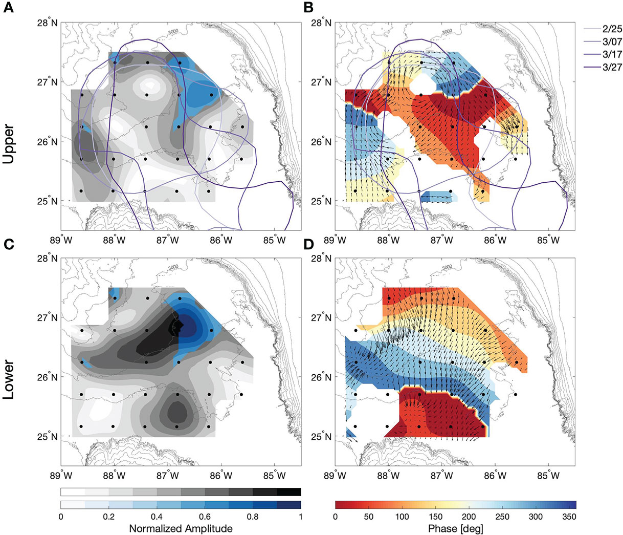
Figure 9 Coupled CEOF from 1/20 – 1/10 day^–1 band-passed baroclinic sea surface height, SSH_bcb (upper) and reference sea surface height, SSH_ref (lower) during LCE Ursa detachment. Normalized spatial amplitude is on the left panels (A, C) and phase in degrees is on the right (B, D). Normalized amplitude is plotted in color only where both the upper and lower exceed 0.4. Phase is plotted only in regions where the spatial amplitude is greater than 0.3. The position of the LC, determined from SSH satellite altimetry, is contoured every 10 days during Ursa detachment on the upper panels. Bathymetry is contoured in gray every 250 meters.

This type of coupling resembles the Malanotte-Rizzoli et al. (1995) theory of forcing TRWs via upper-lower layer resonant coupling. We hypothesize that a near-resonance response is observed in the northeast corner of the array, during short-duration events in which upper layer SSH_bcb meanders propagate with wavenumber and frequency that approximately matches the TRW dispersion relation. This excites fluctuations of similar wavelength and frequency in SSH_ref. When the event evolves away from near-resonant coupling, the deep ocean is nearly unforced and the fluctuations radiate away around the Mississippi Fan as free, unforced TRWs. We will therefore refer to the ‘generation’ and ‘propagation’ regions as the blue highlighted and dark gray regions, respectively, in the lower spatial amplitude coupled CEOF plot (Figure 9C).

To show that this type of resonant coupling can generate TRWs in the Gulf Stream region, Pickart (1995) requires both the frequency and zonal wavelength of the TRWs to match that of the meanders. Additionally, surface meanders must project onto the TRW dispersion relation which, because Gulf Stream meanders are predominantly eastward, requires sufficient northerly orientation of bathymetry at the coupling site to rotate the TRW dispersion relation enough to create an eastward component of phase speed. Here, we have band-passed both SSH_bcb and SSH_ref, confining the frequency of both the upper and lower layer fluctuations to the 1/20 – 1/10 day^–1 band. In this case we require a component of the lower phase speed to match the upper and map onto the TRW dispersion relation local to the bottom slope. The coupled TRW dispersion relation, first derived by Rhines (1970) is:

where k and l are the meridional and zonal wavenumbers, [h_x, h_y] is the topographic slope, h is the local bottom depth, ω is the wave frequency and N is the buoyancy frequency. Here, a constant value of N = 15×10^–4 s^-1 is used, chosen to reflect numerous deep CTD casts across the array. Additionally, the bathymetry is smoothed using a 60-km Gaussian filter to emphasize large bathymetric features expected to influence the generation and propagation of deep waves of wavelength greater than 150 km.

The dispersion relation is calculated by numerically solving for meridional wavenumbers given a range of zonal wavenumbers for a 1/16-day^–1 wave at each bathymetric grid point in a 60-km square box around each CPIES location (Figure 10). This results in a unique dispersion relationship for each bathymetric slope (while keeping frequency and stratification constant) within the 60-km box, giving us the range in dispersion curves for each site in Figure 10. Standard deviation of the zonal and meridional wavenumbers, derived from the coupled CEOF phase, within a 60-km square box around each CPIES site is plotted together with the family of local dispersion curves. In the generation region (blue), both the upper and lower wavevectors are plotted on the dispersion to identify evidence of resonant coupling. In the propagation region (gray), only the lower wavenumber standard deviation is plotted on the dispersion as these waves should be unforced and uncoupled from the surface. Smoothing the bathymetry and calculating the dispersion curves as well as the wavenumbers over a 60-km area was done to capture TRW response to bathymetric features on the order of the observed wavelength. This smoothing is comparable to that done in Oey and Lee (2002). For comparison purposes, the same analysis was done with 30-km smoothing and a 30-km square box (for both dispersion and wavenumbers) and did not yield significantly different results (not shown).

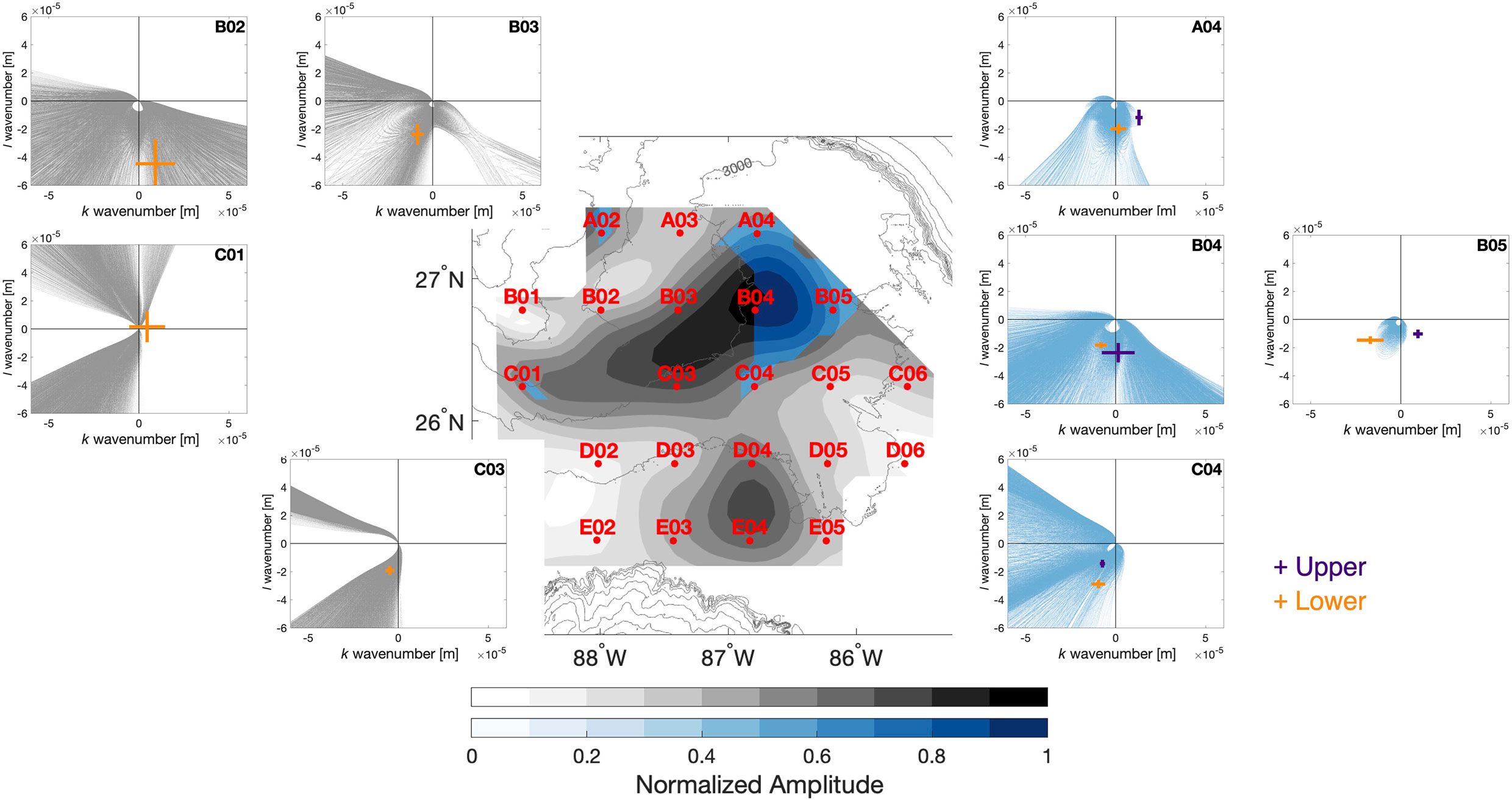
Figure 10 Central panel: normalized spatial amplitude from the coupled CEOF of the 1/20 – 1/10 day^–1 band-passed reference sea surface, SSH_ref, during LCE Ursa detachment (same as Figure 9C). CPIES locations are marked in red and labeled. Bathymetry is contoured in gray every 250 meters. Outside panels: the TRW dispersion curves calculated for each bathymetric slope within a 60-km square kilometer box around the corresponding CPIES sites. To calculate the dispersion relationship, frequency (ω = 1/15 day^–1) and stratification (N = 15×10^–4s^–1) are kept constant across the array and bathymetry is smoothed using a 60-km Gaussian filter. The dispersion relations plotted in blue correspond to sites that fall within the blue region on the spatial amplitude (central) plot and represent regions where we hypothesize TRWs have been generated. The dispersion relations plotted in gray correspond to sites within the region of high spatial amplitude where we hypothesize TRWs are freely propagating. Orange and purple crosses represent the standard deviation of the SSH_ref (lower) and SSH_bcb (upper), respectively, wavevectors local to the corresponding CPIES location.

In the propagation region (Figure 10; gray dispersion diagrams), TRWs are supported for a wide range of wavenumbers. Sites B03 and C03 fall within the band of highest spatial amplitude, appearing to be dominated by TRWs during this time period. The orientation of bathymetry at B03 is northerly while C03 is more northeasterly, allowing for some contrast between the dispersion curves. However, the lower layer southwesterly phase propagation observed from the array falls within the range of TRW dispersion curves suggesting propagation is supported at both locations. On the northern edge of the propagation region, site B02 is located near a bend in bathymetry, generating numerous dispersion curves which support the south to southeastward TRW phase propagation observed. At site C01, bathymetry is aligned nearly east-west and varies only slightly within the 60-km square box, minimizing variance of the dispersion curves. Wavenumbers [k,l] however, are centered close to [0,0] with a relatively large standard deviation in both the zonal and meridional directions. While some of this propagation maps onto the dispersion relation, the large variability indicates more than one process is controlling deep perturbations at site C01.

In the generation region (Figure 10; blue dispersion diagrams), we aim to identify evidence for both TRW propagation and upper-lower layer near-resonant coupling. As in the propagation region, lower layer wavenumbers (orange crosses) are required to map onto the dispersion curve to illustrate that observed perturbations can be attributed to TRWs. Additionally, wavenumbers of upper layer meanders (purple crosses) must, at the very least, have a component in common with lower layer fluctuations and map onto the dispersion curves to satisfy the requirements of near-resonant coupling. In an idealized framework, upper and lower layer wavenumbers would perfectly match each other. However, owing to the variability of the system and likely intermittent coupling over the Ursa time period, we believe a common wavenumber component provides adequate evidence for coupling. Site B04 exemplifies this type of coupling. The upper and lower wavenumbers fall very close to each other, nearly overlapping in the meridional direction with similar magnitude, and also map onto the TRW dispersion relationship. Based on both the joint CEOF and comparison to the dispersion relationship, we believe the strongest coupling is occurring at site B04. At sites A04, C04 and B05, upper and lower wavenumbers share a component in common (mainly southward) suggesting coupling is likely more intermittent at these sites. Coupling may not result in TRWs at site B05 where wavenumbers do not map onto the dispersion curves.

We believe observations from site C01 support a combination of both free and forced waves at this location. Given that spatial amplitude is high and topography appears to act as a wave guide to funnel TRWs through C01 and out the western side of the array, we expected deep phase propagation to fit the dispersion relationship well. However, during both Ursa and other time periods, projection of the local wavenumber onto the dispersion curve is only within the standard deviation limits. This is likely because not only are TRWs propagating through this location but they are also being generated in this region, resulting in both free and forced waves. There is some evidence of coupling from the joint upper-lower layer CEOF (Figure 9C) and just south of C01 there is agreement in phase propagation.

A similar analysis is completed during the time period of LCE Thor to identify TRW pathways and generation regions. A few notable differences between Thor and Ursa made it difficult to draw any definitive conclusions about the origin of high-frequency perturbations observed during Thor. There are two distinct peaks in high-frequency energy associated with each of the detachments over the Thor time period. During the first time period, the generation region appears to be north of the array with perturbations traveling southward before bending around the Mississippi Fan and exiting the array near site C01. We believe a similar coupling mechanism could be responsible for these TRWs, associated with meanders in either the LC or detached LCE. However, because generation is outside the array, the coupled CEOF (not shown) identifies only a single region, site C01, where high amplitudes of both upper and lower layer coincide providing further evidence for a mix of free and forced waves at this location.

7 Summary and conclusions

An array of 24 CPIES deployed in the eastern Gulf of Mexico from June 2019 – May 2021 is well positioned to observe the generation and propagation of TRWs associated with the LC and LCEs. During the two year deployment, three LCEs separate from the core of the LC. Each LCE formation and detachment is associated with a peak in deep eddy kinetic energy under the eastward arm of the LC. This energy is found to organize into two distinct frequency bands, 1/100 – 1/20 days^–1 and 1/20 – 1/10 days^–1, with the high-frequency band dominating over the Mississippi Fan in the northwest corner of the array. We believe this energy to be associated with TRWs generated by LC or LCE interactions with the Mississippi Fan.

A CEOF analysis of 1/20 – 1/10 day^–1 band-passed SSH_ref over the full deployment period identifies a number of characteristics that satisfy linear TRW theory: phase propagation to the right of increasing water depth, current velocity variance ellipses perpendicular to the direction of phase velocity in regions where spatial amplitude is high and a larger phase speed oriented down-slope in regions of steeper bathymetric slope. Additionally, wavelengths of 150 – 300 km are estimated from the phase gradient, values consistent with both linear wave theory and previous observations in the Gulf of Mexico. The time series of EOF coefficients reveals peaks in 1/20 – 1/10 day^–1 energy just following each LCE detachment event as well as a number of smaller peaks seemingly disassociated with the separation process and sometimes occurring during a retracted LC state.

Results from the CEOF analyses strongly suggest observed high-frequency propagation following roughly around the topography of the Mississippi Fan can be attributed to TRWs. This is in agreement with previous works that have identified TRWs at numerous locations across the northern continental slope of the Gulf (Hamilton, 1990; Hamilton and Lugo-Fernandez, 2001; Hamilton, 2007). While many of these studies suggest the LC or LCEs as the source of this deep energy, conclusively linking generation to propagation has proved difficult. A coupled high-frequency SSH_ref (lower layer) and SSH_bcb (upper layer) CEOF during the LCE Ursa formation and detachment time period identifies a TRW propagation region extending from an area where both upper and lower layers exhibit cohesive high amplitude fluctuations. Suggestive of an upper-lower layer resonant coupling mechanism, this is likely a region where high-frequency energy is being generated and radiating away as TRWs within the band of high CEOF amplitude. This region, extending south-southwest and wrapping along the Mississippi Fan suggests the path of group energy propagation. The along path decrease in amplitude likely results from the dispersion of TRW contributions within this band of wavelengths and frequencies.

To illustrate generation by coupling and TRW propagation, wave characteristics are mapped onto the linear dispersion relationship within a 60-km region around each CPIES site. Within the SSH_ref high amplitude fluctuation region, or the propagation region, wavenumbers fit the dispersion curve well, confirming observed perturbations can be attributed to TRWs. In the generation region, upper-lower layer resonant coupling is identified by matching, or having at least one component in common, SSH_ref and SSH_bcb wavenumbers that both map onto the local dispersion curve. In the northeast corner of the array, where the joint CEOF illustrates coherent upper and lower layer fluctuations, site B04 exhibits strong evidence for near-resonance coupling between the upper and lower layers. Coupling is likely more intermittent at the remainder of the sites, where upper and lower wavenumbers share a southward wavenumber. These results provide sufficient evidence for the near-resonant coupling hypothesis.

The CPIES array has identified propagation pathways of high-frequency TRWs around the Mississippi Fan. We believe these waves, generated across the eastern Gulf of Mexico, are likely funneled out of the western side of the array and towards the Sigsbee Escarpment, a known active TRW region. A combination of ray tracing and continuous long term deep current measurements at the Escarpment has the potential to connect generation and propagation within the array to deep hazardous currents that can interfere with energy sector operations.

Data availability statement

The CPIES datasets analyzed for this study can be found in the GRIIDC data repository https://data.gulfresearchinitiative.org/. Specifically, vertical acoustic round trip travel time: https://data.gulfresearchinitiative.org/data/U1.x852.000:0005 and DOI:10.72664B13NKBA, vertical profiles of temperature, salinity and geopotential anomaly: https://data.gulfresearchinitiative.org/data/U1.x852.000:0007 and DOI:10.7266GE30701Z, bottom pressure: https://data.gulfresearchinitiative.org/data/U1.x852.000:0004 and DOI:10.7266BZ9B3C54, and bottom current meter data: https://data.gulfresearchinitiative.org/data/U1.x852.000:0003 and DOI:10.7266K4ZF1T9Z. The mapped altimeter SSH product can be found at https://resources.marine.copernicus.eu/product-detail/SEALEVEL _GLO_pHY_L4_NRT_OBSERVATIONS₀08₀46/INFORMATION.

Author contributions

AJE, KD, and DW contributed to conception and design of the study. KT and MK processed and organized the database. AJE performed the statistical analysis and wrote the first draft of the manuscript. All authors contributed to manuscript revision, read, and approved the submitted version.

Funding

Funding for this project was provided by the National Academy of Science, Engineering and Medicine Grant 2000009943.

Acknowledgments

The authors would like to thank the Captain, Tad Berkey, and crew of the R/V Pelican for the successful deployment and recovery of the array. We also acknowledge instrument development and careful planning and preparation by Erran Sousa and Laura Reed. This paper has benefited from the thoughtful comments from the editor, Julio Sheinbaum.

Conflict of interest

The authors declare that the research was conducted in the absence of any commercial or financial relationships that could be construed as a potential conflict of interest.

Publisher’s note

All claims expressed in this article are solely those of the authors and do not necessarily represent those of their affiliated organizations, or those of the publisher, the editors and the reviewers. Any product that may be evaluated in this article, or claim that may be made by its manufacturer, is not guaranteed or endorsed by the publisher.

References

Bretherton F. P., Davis R. E., Fandry C. (1976). ). a technique for objective analysis and design of oceanographic experiments applied to MODE-73. Deep Sea Res. 23, 559–582. doi: 10.1016/0011-7471(76)90001-2
Donohue K., Hamilton P., Leaman K., Leban R., Prater M., Waddell E., et al. (2006). Exploratory study of deepwater currents in the gulf of Mexico, volume 2: Technical report (Tech. rep., United States. Minerals Management Service. Gulf of Mexico OCS Region). Available at: https://digital.library.unt.edu/ark:/67531/metadc955399/.
Donohue K. A., Watts D., Hamilton P., Leben R., Kennelly M. (2016). Loop current eddy formation and baroclinic instability. dyn. atmos. Oceans 76, 195–216. doi: 10.1016/j.dynatmoce.2016.01.004
Donohue K. A., Watts D. R., Tracey K. L., Greene A. D., Kennelly M. (2010). Mapping circulation in the kuroshio extension with an array of current and pressure recording inverted echo sounders. J. Atmos. Oceanic Technol. 27, 507–527. doi: 10.1175/2009JTECHO686.1
Hamilton P. (1990). Deep currents in the gulf of Mexico. J. Phys. Oceanogr. 20, 1087–1104. doi: 10.1175/1520-0485(1990)020<1087:DCITGO>2.0.CO;2
Hamilton P. (2007). Deep-current variability near the sigsbee escarpment in the gulf of Mexico. J. Phys. Oceanogr. 37, 708–726. doi: 10.1175/JPO2998.1
Hamilton P. (2009). Topographic rossby waves in the gulf of Mexico. Prog. Oceanogr. 82, 1–31. doi: 10.1016/j.pocean.2009.04.019
Hamilton P., Bower A., Furey H., Leben R., Pérez-Brunius P. (2019). The loop current: Observations of deep eddies and topographic waves. J. Phys. Oceanogr. 49, 1463–1483. doi: 10.1175/JPO-D-18-0213.1
Hamilton P., Donohue K., Hall C., Leben R., Quian H., Sheinbaum J., et al. (2015). Observations and dynamics of the loop current (Tech. rep., US Department of the Interior, Bureau of Ocean Energy Management, Gulf of Mexico OCS Region). Available at: https://digital.library.unt.edu/ark:/67531/metadc955416/.
Hamilton P., Lugo-Fernandez A. (2001). Observations of high speed deep currents in the northern gulf of Mexico. Geophys. Res. Lett. 28, 2867–2870. doi: 10.1029/2001GL013039
Hirschi J. J.-M., Frajka-Williams E., Blaker A. T., Sinha B., Coward A., Hyder P., et al. (2019). Loop current variability as trigger of coherent gulf stream transport anomalies. J. Phys. Oceanogr. 49, 2115–2132. doi: 10.1175/JPO-D-18-0236.1
Kennelly M., Tracey K., Donohue K., Watts D. R. (2022). PIES and CPIES data processing manual (Tech. rep., University of Rhode Island Graduate School of Oceanography). Available at: https://digitalcommons.uri.edu/cgi/viewcontent.cgi?article=1037&context=physical_oceanography_techrpts.
Le Hénaff M., Kourafalou V. H., Morel Y., Srinivasan A. (2012). Simulating the dynamics and intensification of cyclonic loop current frontal eddies in the gulf of Mexico. J. Geophys. Res. 117. doi: 10.1029/2011JC007279
Malanotte-Rizzoli P., Dale B. H., Young R. E. (1987). Numerical simulation of transient boundary-forced radiation. part I: The linear regime. J. Phys. Oceanogr. 17, 1439–1457. doi: 10.1175/1520-0485(1987)017<1439:NSOTBF>2.0.CO;2
Malanotte-Rizzoli P., Hoggi N. G., Young R. E. (1995). Stochastic wave radiation by the gulf stream: Numerical experiments. Deep Sea Res. 42, 389–423. doi: 10.1016/0967-0637(95)00001-M
Meinen C. S., Watts D. R. (2000). Vertical structure and transport on a transect across the north Atlantic current near 42 n: Time series and mean. J. Geophys. Res. 105, 21869–21891. doi: 10.1029/2000JC900097
Munk W. H., Cartwright D. E. (1966). Tidal spectroscopy and prediction. Philos. Trans. R. Soc. London 259, 533–581. doi: 10.1098/rsta.1966.0024
Oey L. (2008). Loop current and deep eddies. J. Phys. Oceanogr. 38, 1426–1449. doi: 10.1175/2007JPO3818.1
Oey L., Lee H. (2002). Deep eddy energy and topographic rossby waves in the gulf of Mexico. J. Phys. Oceanogr. 32, 3499–3527. doi: 10.1175/1520-0485(2002)032<3499:DEEATR>2.0.CO;2
Pickart R. S. (1995). Gulf stream–generated topographic rossby waves. J. Phys. Oceanogr. 25, 574–586. doi: 10.1175/1520-0485(1995)025<0574:GSTRW>2.0.CO;2
Rhines P. (1970). Edge-, bottom-, and rossby waves in a rotating stratified fluid. Geophys. Fluid Dyn. 1, 273–302. doi: 10.1080/03091927009365776
Trenberth K. E., Shin W.-T. K. (1984). Quasi-biennial fluctuations in sea level pressures over the northern hemisphere. Monthly Weather Rev. 112, 761–777. doi: 10.1175/1520-0493(1984)
Watts D. R., Qian X., Tracey K. L. (2001). Mapping abyssal current and pressure fields under the meandering gulf stream. J. Atmos. Oceanic Technol. 18, 1052–1067. doi: 10.1175/1520-0426(2001)018<1052:MACAPF>2.0.CO;2
Keywords: topographic Rossby waves, Gulf of Mexico, Loop Current, deep energy propagation, inverted echo sounders, deep currents
Citation: Johnson Exley A, Donohue KA, Watts D R, Tracey KL and Kennelly MA (2022) Generation of high-frequency topographic Rossby waves in the Gulf of Mexico. Front. Mar. Sci. 9:1049645. doi: 10.3389/fmars.2022.1049645
Received: 20 September 2022; Accepted: 07 December 2022;
Published: 22 December 2022.
Edited by:
Julio Sheinbaum, Centro de Investigación Científica y de Educación Superior de Ensenada (CICESE), MexicoCopyright © 2022 Johnson Exley, Donohue, Watts, Tracey and Kennelly. This is an open-access article distributed under the terms of the Creative Commons Attribution License (CC BY). The use, distribution or reproduction in other forums is permitted, provided the original author(s) and the copyright owner(s) are credited and that the original publication in this journal is cited, in accordance with accepted academic practice. No use, distribution or reproduction is permitted which does not comply with these terms.
*Correspondence: Alexis Johnson Exley, ajohnson1@uri.edu